Content from What is an HPC cluster?
Last updated on 2025-10-21 | Edit this page
Estimated time: 20 minutes
Overview
Questions
- What is an HPC cluster?
- When would you use HPC instead of a laptop?
- How does HPC allocate resources to your job?
Objectives
- Explain some advantages and disadvantages of HPC over laptop
- Explain some different types of HPC job
- Understand that HPC uses a scheduler to run jobs
Motivation
Some research computation is not suitable for running on your laptop—maybe it takes too long to run, needs more memory than you have available on your laptop, or uses too much disk space.
These types of problems needn’t be a limitation on the research you can do, if you have access to a High Performance Computing (HPC) cluster.
We will first discuss working on a laptop before looking at what HPC entails.
Using a laptop
This is a familiar set up, is accessed locally, and the user can run a GUI right away. However, laptops have some significant limitations for research computing.
Let’s imaging that you have a resource-intensive job to run—perhaps a simulation, or some data analysis. You might be able to do this using a laptop, but it requires your laptop to be left on, and probably precludes you from using it for much else until the job has finished.
You are likely also limited to only one “job” (simulation/analysis) at a time.
Consider the schematic below that represents typical resources you might have on a laptop—4 cores (CPUs) and 8GB of memory.

Using HPC
When logged in to an HPC cluster, things look a bit different.
Your work, or “jobs” must be submitted to a scheduler, and wait in a queue until resources are available.
Jobs run on high-end hardware, so you have access to lots of cores and memory. You can log out of the cluster while the jobs run, and many jobs can run at once.
Let’s now consider the HPC schematic below.

Users connect to the HPC system via a login node. This is a shared resource where users can submit batch (non-interactive) jobs. You shouldn’t run work on the login node as this will make the login node slow for other users.
Jobs don’t (usually) run immediately, rather jobs must be submitted to the job scheduler, which decides which compute node(s) will run the job.
“Nodes” are a bit like high-end workstations (lots of CPUs (cores) and memory), linked together to make up a cluster. A cluster will typically have many nodes, suitable for varying types of job.
Compute nodes actually do the computation, and have (high performance) resources specifically allocated for the job.
Your files can be stored in your home directory (which is backed up) but jobs are usually submitted from scratch, which is a faster file system with more storage, though files here aren’t usually backed up.
Types of HPC jobs
An HPC cluster is usually composed of multiple types of hardware, each of which lend themselves to different types of jobs.
The simplest type of HPC job is a serial job, which uses 1 CPU to complete the work.
High Performance Computing (HPC) describes solving computationally intensive problems quickly. This usually involves powerful CPUs and parallel processing (splitting work over multiple CPUs, or even over multiple nodes).
High Throughput Computing (HTC) means running the same task on multiple different inputs. The tasks are independent of each other so can be run at the same time. This might be processing multiple data files, or running simultions using different input parameter values each time.
Graphics Processing Units (GPUs) lend themselves well to tasks that involve a lot of matrix multiplication such as image processing, machine learning, and physics simulations.
High Memory jobs use CPUs that have lots of memory available to them—these can be serial or parallel tasks.
Challenge 1: What are some pros and cons of using an HPC cluster?
- laptop takes too long to run/ needs more memory/ uses too much disk space
- HPC jobs can run for days without you logged in
- can run multiple jobs at once
- can run on high end hardware (lots of cores/memory/GPU)
- types of HPC jobs (HTC, multi-core, multi-node (MPI), GPU)
Content from Connecting to an HPC system
Last updated on 2025-12-15 | Edit this page
Estimated time: 40 minutes
Overview
Questions
- How do I connect to an HPC cluster?
Objectives
- Be able to use
sshto connect to an HPC cluster - Be aware that some IDEs can be configured to connect using
ssh
Connecting to the HPC cluster
We learned in the previous episode that we access a cluster via the
login node, but not how to. We will use an encrypted network protocol
called ssh (secure shell) to connect, and the usual way to
do this is via a terminal (also known as the command line or shell).
The shell is another way to interact with your computer instead of a Graphical User Interface (GUI). Instead of clicking buttons and navigating menus, you give instructions to the computer by executing commands at a prompt, which is a sequence of characters in a Command Line Interface (CLI) which indicates readiness to accept commands.
One of the advantages of a CLI is the ability to chain together commands to quickly create custom workflows, and automate repetitive tasks. A CLI will typically use fewer resources than a GUI, which is one of the reasons they’re used in HPC. A GUI can be more intuitive to use, but you’re more limited in terms of functionality.
There are pros and cons of GUIs vs CLIs (command line interface), but suffice to say that a CLI is how you interact with an HPC cluster.
We’ll first practice a little bit with the CLI by looking at the files on our laptops.
Open your terminal/Git Bash now and you’ll see that there is a prompt. This is usually something like:
The information before the $ in the example above shows
the logged in user (you) and the hostname of
the machine (laptop), and the working directory
(~). Your prompt may include something different (or
nothing) before the $, and might finish with a different
character such as # instead of $.
There is very likely a flashing cursor after your prompt – this is where you type commands. If the command takes a while to run, you’ll notice that your prompt disappears. Once the command has finished running, you’ll get your prompt back again.
Let’s run a couple of commands to view what is in our home directory:
The cd command changes the “working directory” which is
the directory where the shell will run any commands. Without any
arguments, cd will take you to your home directory. You can
think of this like a default setting for the cd
command.
Now we’re going to list the contents of our home directory.
OUTPUT
Desktop  Documents  Downloads  Music  Pictures  Public  Videos
[you@laptop ~]$ cd
Your output will look different but will show the contents of your home directory. Notice that after the output from the command is printed, you get your prompt back.
Where is your home directory? We can print the current working directory with:
OUTPUT
/home/usernameAgain, your output will look slightly different. When using a UNIX
type system such as Linux or macOS, the directory structure can be
thought of as an inverse tree, with the root directory / at
the top level, and everything else branching out beneath that. Git Bash
(or another terminal emulator) will treat your file system similarly,
with the hard drive letter showing as a directory so your home directory
would be something like:
OUTPUT
/c/users/you/homeLet’s now connect to the HPC cluster, using the username and password emailed to you for this course, i.e. not your normal university username:
Forgotten your password?
Reset it here using your email address:
https://hpc-training.digitalmaterials-cdt.ac.uk:8443/reset-password/step1
If this is your first time connecting to the cluster, you will see a message like this:
OUTPUT
The authenticity of host 'hpc-training.digitalmaterials-cdt.ac.uk (46.62.206.78)' can't be established.
ED25519 key fingerprint is SHA256:..........
This key is not known by any other names.
Are you sure you want to continue connecting (yes/no/[fingerprint])?
This is normal and expected, and just means that your computer hasn’t
connected to this server before. Type yes and then you will
see something like this:
OUTPUT
Warning: Permanently added 'hpc-training.digitalmaterials-cdt.ac.uk' (ED25519) to the list of known hosts.At this point you will be prompted for your password. As you enter it you won’t see anything you type, so type carefully.
Once you’ve logged in you should see that your prompt changes to something like:
Bear in mind that other HPC systems are likely to have a slightly different prompt – some examples are given below:
Note that while the values are different, it usually follows broadly the same pattern as the prompt on your laptop, showing your username, the hostname of the login node, and your current directory.
The command needed to connect to your local institution’s cluster
will look similar to the ssh command we just used, but each
HPC system should have documentation on how to get an account and
connect for the first time e.g. Manchester’s CSF
and the ARCHER2
national cluster.
Your home directory will usually be at a different location:
OUTPUT
/some/path/yourUsernameand it will contain different files and subdirectories (but might be empty if you’ve not logged in before):
Git Bash isn’t the only tool you can use to connect to HPC from Windows. MobaXterm is a popular tool with a CLI and some graphical tools for file transfer.
VScode can be configured for ssh, but follow instructions for configuring VScode so it doesn’t hog resources on the login node! e.g. https://ri.itservices.manchester.ac.uk/csf3/software/tools/vscode/
Explore resources on the cluster
A typical laptop might have 2-4 cores and 8-16GB of RAM (memory). You laptop might have a bit more or a bit less, but we’ll use this as a reference to compare with the resources on the HPC cluster.
Explore resources on the login node
We have already considered the resources of a typical laptop – how does that compare with the login node?
You should already be connected to the HPC cluster, but if not log back in using:
See how many cores and how much memory the login node has, using the
commands below. nproc gives the numer of CPUs, and
free -gh shows available memory.
You can get more information about the processors using
lscpu
The output from the commands is shown below, which tells us that the login node has 4 cores and 15GB of memory, which is comparable to a typical laptop.
BASH
userName@login:~$ nproc
4
userName@login:~$ free -gh
              total        used        free      shared  buff/cache   available
Mem:           15Gi       401Mi        11Gi       5.0Mi       3.7Gi        14Gi
Swap:            0B          0B          0B
The login node on most clusters will have more CPUs and memory than your laptop, although as we will soon see, the compute nodes will have even more cores and RAM than the login nodes.
As noted in the setup section the cluster used for this course is an exception to this rule, and has very little computing resource.
Your output should show something that looks a bit like this:
OUTPUT
HOSTNAMES  CPUS  MEMORY
compute01  4     15610
On most clusters you’re likely to see a few different types of compute node with different numbers of cores and memory, e.g.
OUTPUT
HOSTNAMES  CPUS  MEMORY
node1203   168   1546944
node1204   168   1546944
node1206   168   1546944
node1207   168   1546944
node1208   168   1546944
node904    32    191520
node600    24    128280
node791    32    1546104
node868    48    514944
node870 48 514944Compare a laptop, the Login Node and the Compute Node
Consider the output below from a typical HPC cluster, rather than the numbers you got from the cluster used for this training course.
OUTPUT
96OUTPUT
               total        used        free      shared  buff/cache   available
Mem:           754Gi        50Gi       216Gi       1.2Gi       495Gi       704Gi
Swap:           15Gi          0B        15Gi
Compare your laptop’s number of processors and memory with the numbers from a typical HPC system’s login node (above) and compute nodes (below).
OUTPUT
HOSTNAMES  CPUS  MEMORY
node1203   168   1546944  # Units is MB, so  roughly 1.5TB
node1204   168   1546944
node1206   168   1546944
node1207   168   1546944
node1208   168   1546944
node904    32    191520
node600    24    128280
node791    32    1546104
node868    48    514944
node870    48    514944
What implications do you think the differences might have on running your research work on the different systems and nodes?
Compute nodes are usually built with processors that have higher core-counts than the login node or personal computers in order to support highly parallel tasks. Compute nodes usually also have substantially more memory (RAM) installed than a personal computer. More cores tends to help jobs that depend on some work that is easy to perform in parallel, and more, faster memory is key for large or complex numerical tasks.
- The
sshprotocol is used to connect to HPC clusters - The cluster should have documentation detailing how to connect
Content from The job scheduler
Last updated on 2025-12-15 | Edit this page
Estimated time: 45 minutes
Overview
Questions
- What is a job scheduler?
- How do I run a program on HPC?
- How do I check on a submitted job or cancel it?
Objectives
- Be able to navigate the filesystem
- Submit a serial job to the scheduler
- Monitor the execution status of jobs (running/waiting/finished/failed)
- Inspect the output and error files from a job
- Find out how long your job took to run and what resources it used
An HPC system might have thousands of nodes and thousands of users. How do we decide who gets what and when? How do we ensure that a task is run with the resources it needs? This job is handled by a special piece of software called the scheduler. On an HPC system, the scheduler manages which jobs run where and when.
We will be using the SLURM scheduler, which is probably the most widely used scheduler for HPC, but many of the concepts we’ll encounter are transferable to other scheduler software you might encounter when using HPC, such as SGE.
Users interact with the scheduler using a jobscript, which is plain text file containing commands to be run, and requests for computing resources e.g. how much time, memory, and CPUs the job can use.
Jobscripts are usually submitted from the scratch
filesystem, because it has more space and reads/writes files more
quickly. Our training cluster doesn’t have a scratch
filesystem, so for this course we’ll work in our home directories
instead.
Submitting a jobscript
The first step we’re going to take towards writing a jobscript is to write a small shell script – essentially a text file containing a list of UNIX commands to be executed in a sequential manner.
We’ll use a command-line text editor called nano to
create this file. This is a fairly intuitive, light weight text editor
that is widely available.
This starts a CLI text editor that looks like this:
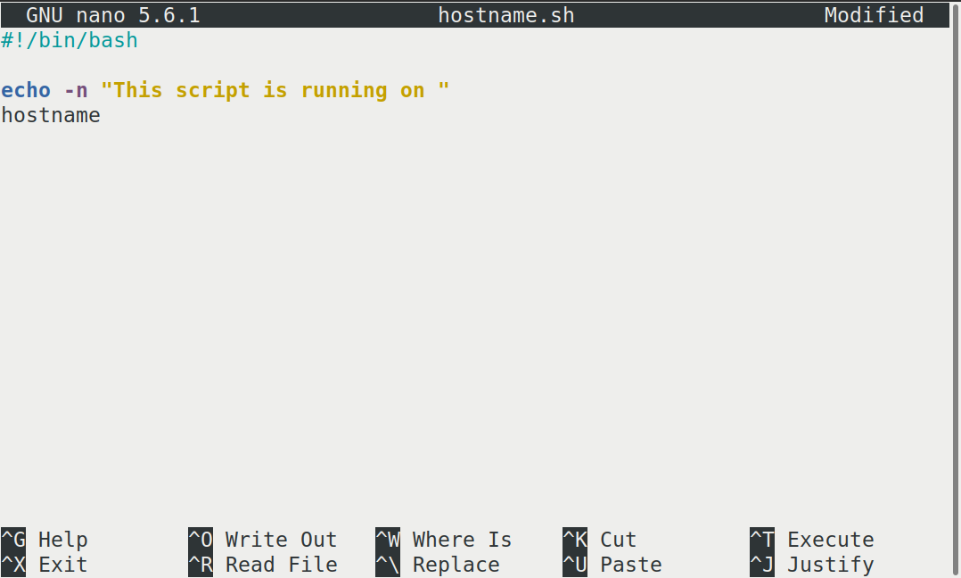
Our shell script will have three parts:
- On the very first line, add
#!/bin/bash. The#!(pronounced “hash-bang” or “shebang”) tells the computer what program is meant to process the contents of this file. In this case, we are telling it that the commands that follow are written for the Bash shell. All characters after a#symbol in a shell script are treated as comments (i.e. for information only) and are not executed as commands. Most commonly, comments are written for the benefit of someone reading the script, but the shebang can be thought of as a special type of comment for the computer to read. - Anywhere below the first line, we’ll add an
echocommand with a friendly greeting. When run, the shell script will print whatever comes after echo in the terminal.echo -nwill print everything that follows, without ending the line by printing the new-line character. - On the last line, we’ll invoke the
hostnamecommand, which will print the name of the machine the script is run on.
When finished the file should look like this:
#!/bin/bash

echo -n "This script is running on "
hostname
To close the editor when finished, we use the keyboard shortcuts shown at the bottom of the screen: Ctrl+O to save (Write Out), followed by Return to confirm the file name, and then Ctrl+X to exit.
Mac users also need to use Ctrl rather than CMD.
The shebang isn’t needed to run the shell script with
bash hostname.sh, but is needed for the SLURM jobscript.
It’s probably still a good practice to include it, but certainly not
worth explaining permissions to make a script executable.
If a question comes up about this it might be good to show that the jobscript won’t submit without it.
Ok, so we’ve written a shell script—how do we run it? You might be familiar with other scripting languages such as python, and be familiar with running a python script using something like :
We can do similar with our shell script, and run it using
Challenge
If you haven’t already, run the shell script
hostname.sh. Does it execute on the cluster or just our
login node?
This script ran on the login node, but we want to take advantage of
the compute nodes: we need the scheduler to queue up
hostname.sh to run on a compute node.
To submit a jobscript to the scheduler, we use the SLURM
sbatch command. This creates a job which will run the
script when dispatched to a compute node which the queuing system has
identified as being available to perform the work.
A jobscript should normally contain some SLURM directives to tell the scheduler something about the resources we want available for the job e.g. how many cores to allocate, a time limit, and what type of job this is (e.g. serial, parallel, high memory etc)
Our shell script doesn’t yet contain any of this information for the job scheduler, so we wouldn’t expect it to work.
We can try submitting it anyway—let’s see what happens.
The command we’re going to need is sbatch hostname.sh,
which we could just type out, but there is a shortcut. We’ll
start by typing sbatch h, then press the Tab
key. This will show us a list of possible matches starting with the
letter h, or complete the file name for us if there is only
one match.
This is called tab-completion, and can be used to complete the names of files and directories, in addition to commands. Not only does this make your typing quicker, it also reduces typos because it can only complete file and command names that exist.
OUTPUT
Submitted batch job 340The training cluster we are using has some default settings for SLURM, so our job submitted without errors, but in general, for your job to run correctly, you will need to tell the scheduler which partition to use, how many cores, and specify a time limit for your job. Failure to provide enough information results in an error like the one below:
OUTPUT
sbatch: error: Batch job submission failed: Invalid partition name specifiedThe SLURM partitions are equivalent to job queues for different types of jobs e.g. serial, parallel, GPU, high memory etc that we encountered in the introduction section).
We’ll supply the missing information by editing the jobscript. We
could use tab completion again to speed up typing
nano hostname.sh by using nano h +
Tab, or another shortcut is to use the up arrow key
↑ to cycle through previous commands until we get the one we
want.
BASH
#!/bin/bash
#SBATCH -p compute     # The name of the available partitions varies between clusters
#SBATCH -t 2           # Set a time limit of 2 minutes


echo -n "This script is running on "
hostname
The shebang line must be the first line of the jobscript, so we add
our SLURM directives underneath the initial shebang line, but
above the commands we want to run as our job. The directives start with
#SBATCH and are essentially a special type of
comment which is interpreted by the SLURM software. The first
directive is #SBATCH -p to specify which partition we want
to use. Partitions can be listed using the SLURM command
sinfo, but the cluster documentation will normally explain
when to use each partition. The second directive #SBATCH -t
indicates a time limit for our job.
Now that we have a jobscript with SLURM directives, let’s check that we’ve not made any errors by submitting it to the scheduler again:
We should see something like this that indicates the job has been submitted to the scheduler.
OUTPUT
Submitted batch job 2461232We can check on the status of a running job using the
squeue command.
OUTPUT
JOBID PARTITION NAME USER ST TIME NODES NODELIST(REASON)There are no jobs listed (only the column headings), so we can logically assume that our jobs have either completed successfully, or failed.
Where’s the output from the test job?
When we ran our shell script on the login node, we saw output in the terminal telling us which node the job was running on.
You’ll notice that you don’t see any output printed to the terminal as your jobscript runs. Where does the output go?
Cluster job output is typically redirected to a file in the directory
you submitted it from. Use ls to find and nano
to view the file.
Your output should be in a file called
slurm-[JOB_ID].out. One way to view the contents is with
nano slurm-[JOB-ID].out, or to print the contents in your
terminal, use cat slurm-[JOB-ID].out.
Checking on a job
Check on the status of a submitted job
Edit the hostname.sh script to add a sleep
time of 1 minute. This will give you enough time to check on the job
before it finishes running. Submit the jobscript again, then run
squeue to view the status of the submitted job.
Your test jobscript should look like this:
The output from squeue will look a bit like this:
OUTPUT
JOBID PARTITION     NAME     USER ST       TIME  NODES NODELIST(REASON)
  173   compute hostname username  R       0:02      1 compute01
We’ve already encountered some of the column headings such as the job
ID, and SLURM partition, and we can reasonably expect NAME
to refer to the name of the job (defaults to the jobscript file name if
you’ve not explicitly given a name).
ST means status and displays the job state
code. Common codes include R for running,
CA for cancelled, CD for completed,
PD for pending (waiting for resources), and F
for failed.
TIME refers to how long the job has been running for,
NODES shows how many nodes the job is running on, and
NODELIST lists the nodes the job is running on. If it
hasn’t started yet, a reason is given in brackets such as
(Priority) meaning that other users have higher priority,
or (Resources) which means that resources are not currently
available for your job.
Cancel a running job
Sometimes you’ll realise there is a problem with your job soon after submitting it.
In this scenario it is usually preferable to cancel the job rather than let it complete with errors, or produce output that is incorrect. It is also less wasteful of resources.
Resubmit your hostname.sh jobscript. View the status
(and job ids) of your running jobs using squeue
(JOBID is the first column).
Make a note of the job id of your hostname.sh then
cancel the job using
before it finishes.
Verify that the job was cancelled by looking at the job’s log file,
slurm-[job-id].out.
Your output should look similar to this:
yourUsername@login:~$ sbatch hostname.sh
Submitted batch job 332
yourUsername@login:~$ squeue
             JOBID PARTITION     NAME     USER ST       TIME  NODES NODELIST(REASON)
               332   compute hostname username  R       0:02      1 compute01
yourUsername@login:~$ scancel 332
yourUsername@login:~$ cat slurm-332.out
This script is running on compute01
slurmstepd-compute01: error: *** JOB 332 ON compute01 CANCELLED AT 2025-10-13T12:53:19 ***
Check the status of a completed job
squeue shows jobs that are running or waiting to run,
but to view all jobs including those that have finished or failed, we
need to use sacct.
Run sacct now to view all the jobs you have submitted so
far.
Running sacct shows the job ID and some statistics about
your jobs.
For now we are most interested in the State column—the examples so far in the course should result in at least one job with each of the states “COMPLETED”, “CANCELLED”, and “TIMEOUT”.
Other statuses you might see include “RUNNING”, “PENDING”, or “OUT_OF_MEMORY”.
OUTPUT
       JobID    JobName  Partition    Account  AllocCPUS      State ExitCode
------------ ---------- ---------- ---------- ---------- ---------- --------
330          hostname.+    compute     (null)          0  COMPLETED      0:0
331          hostname.+    compute     (null)          0    TIMEOUT      0:0
332          hostname.+    compute     (null)          0  CANCELLED      0:0
Resource requests
Resource requests (e.g. time limit, number of CPUs, memory) are typically binding. If you exceed them, your job will be killed i.e. automatically cancelled by the scheduler. Let’s use wall time as an example. We will request 1 minute of wall time, and attempt to run a job for two minutes.
Let’s edit the third and 5th line of the jobscript to make these changes:
BASH
#!/bin/bash
#SBATCH -p compute     # The name of the available partitions varies between clusters
#SBATCH -t 1           # Set a time limit of 1 minute

sleep 120              # time in seconds
echo -n "This script is running on "
hostname
and resubmit the jobscript and wait for it to finish:
We can then view the status of the job using sacct — the
most recent job should have the status of “TIMEOUT”. Something like
this:
BASH
yourUsername@login:~$ sacct
       JobID    JobName  Partition    Account  AllocCPUS      State ExitCode
------------ ---------- ---------- ---------- ---------- ---------- --------
102          hostname.+    compute     (null)          0    TIMEOUT      0:0
We can also check the log file by printing it using
cat:
BASH
yourUsername@login:~$ cat slurm-[JobID].out
This script is running on compute01
slurmstepd-compute01: error: *** JOB 178 ON compute01 CANCELLED AT 2025-10-09T10:14:17 DUE TO TIME LIMIT ***
Our job was killed for exceeding the amount of resources it requested. Although this appears harsh, this is actually a good feature. Strict adherence to resource requests allows the scheduler to find the best possible place for your jobs. Even more importantly, it ensures that another user cannot use more resources than they’ve been given. If another user messes up and accidentally attempts to use all of the cores or memory on a node, Slurm will either restrain their job to the requested resources or kill the job outright. Other jobs on the node will be unaffected. This means that one user cannot mess up the experience of others – the only jobs affected by a mistake in scheduling will be their own.
It is a good idea to request slightly more resources than you expect
to need. If you request a lot more (e.g. time) than your job needs it
will likely sit in the scheduler queue for longer. You can get some idea
of the likely resources required from previous, similar jobs you have
submitted—sacct usually outputs more details than on our
training cluster.
Time formats
We have previously used the -t 2 option to request 2
minutes. There are multiple acceptable formats
possible to specify the time limit: “minutes”, “minutes:seconds”,
“hours:minutes:seconds”, “days-hours”, “days-hours:minutes” and
“days-hours:minutes:seconds”.
Interactive jobs
Most of the work done on HPC tends to be batch jobs, where you submit your jobscript to the scheduler and you have no further interaction with it while it runs.
Sometimes you need to run a task interactively e.g. using a GUI, or perhaps you’re debugging a failed job, or testing a small example before submitting a batch job.
These are typically not suitable tasks to run on the login node as they’re too resource-intensive, so usually there is an interactive partition which will enable you to use a compute node directly for a limited time period.
The details vary between HPC clusters, but will use some variation on
the srun command. Check the documentation for your HPC
cluster to find out how to do this.
- A jobscript is a shell script containing SLURM commands in addition to the commands you want to run
- Submit your jobscript using
sbatch - Run your jobs from the “scratch” filesystem
- Request slightly more resources than you will need
Content from Transferring files
Last updated on 2025-10-15 | Edit this page
Estimated time: 35 minutes
Overview
Questions
- How do I transfer files to and from an HPC cluster?
Objectives
- Copy files from your laptop onto the cluster (and vice-versa)
- Download files directly onto the cluster
Performing work on a remote computer is not very useful if we cannot get files to or from the cluster. There are several options for transferring data between computing resources using CLI and GUI utilities, a few of which we will cover.
Download Lesson Files From the Internet Onto Your Laptop
One of the most straightforward ways to download files is to use
either curl or wget. One of these is usually
installed in most Linux shells, on Mac OS terminal and in GitBash. Any
file that can be downloaded in your web browser through a direct link
can be downloaded using curl or wget. This is
a quick way to download datasets or source code. The syntax for these
commands is
BASH
wget [-O new_name] https://some/link/to/a/file
curl [-o new_name] -L https://some/link/to/a/file
By default, curl and wget download files to
the same name as the file on the remote file server. The -O
option to wget and the -o option to
curl allow you to specify a new name for the file that you
download.
Note that curl needs the -L option to
follow links that redirect, whereas wget follows follows by
default.
Download the “tarball””
Try it out by downloading some material we’ll use later on, from a terminal on your local machine, using the URL of the current codebase:
https://github.com/hpc-carpentry/amdahl/tarball/main
The word “tarball” in the above URL refers to a compressed archive
format commonly used on Linux, which is the operating system the
majority of HPC cluster machines run. A tarball is a lot like a
.zip file. The actual file extension is
.tar.gz, which reflects the two-stage process used to
create the file: the files or folders are merged into a single file
using tar, which is then compressed using
gzip, so the file extension is “tar-dot-g-z.” That’s a
mouthful, so people often say “the xyz tarball” instead.
You may also see the extension .tgz, which is just an
abbreviation of .tar.gz.
Use one of the above commands to save the tarball as
amdahl.tar.gz, rather than using the same name as on the
server
[you@laptop:~]$ wget -O amdahl.tar.gz https://github.com/hpc-carpentry/amdahl/tarball/main
# or
[you@laptop:~]$ curl -o amdahl.tar.gz -L https://github.com/hpc-carpentry/amdahl/tarball/main
After downloading the file, use ls to see it in your working directory:
Archiving Files
One of the biggest challenges we often face when transferring data between remote HPC systems is that of large numbers of files. There is an overhead to transferring each individual file and when we are transferring large numbers of files these overheads combine to slow down our transfers to a large degree.
The solution to this problem is to archive multiple files into
smaller numbers of larger files before we transfer the data to improve
our transfer efficiency. Sometimes we will combine archiving with
compression to reduce the amount of data we have to transfer and so
speed up the transfer. The most common archiving command you will use on
a (Linux) HPC cluster is tar.
tar can be used to combine files and folders into a
single archive file and optionally compress the result. Let’s look at
the file we downloaded from the lesson site,
amdahl.tar.gz.
The .gz part stands for gzip, which is a
compression library. It’s common (but not necessary!) that this kind of
file can be interpreted by reading its name: it appears somebody took
files and folders relating to something called “amdahl,” wrapped them
all up into a single file with tar, then compressed that
archive with gzip to save space.
Let’s see if that is the case, without unpacking the file.
tar prints the “table of contents” with the -t
flag, for the file specified with the -f flag followed by
the filename. Note that you can concatenate the two flags: writing
-t -f is interchangeable with writing -tf
together. However, the argument following -f must be a
filename, so writing -ft will not work.
BASH
[you@laptop:~]$ tar -tf amdahl.tar.gz
hpc-carpentry-amdahl-46c9b4b/
hpc-carpentry-amdahl-46c9b4b/.github/
hpc-carpentry-amdahl-46c9b4b/.github/workflows/
hpc-carpentry-amdahl-46c9b4b/.github/workflows/python-publish.yml
hpc-carpentry-amdahl-46c9b4b/.gitignore
hpc-carpentry-amdahl-46c9b4b/LICENSE
hpc-carpentry-amdahl-46c9b4b/README.md
hpc-carpentry-amdahl-46c9b4b/amdahl/
hpc-carpentry-amdahl-46c9b4b/amdahl/__init__.py
hpc-carpentry-amdahl-46c9b4b/amdahl/__main__.py
hpc-carpentry-amdahl-46c9b4b/amdahl/amdahl.py
hpc-carpentry-amdahl-46c9b4b/requirements.txt
hpc-carpentry-amdahl-46c9b4b/setup.py
This example output shows a folder which contains a few files, where
46c9b4b is an 8-character git commit hash that will change
when the source material is updated.
Now let’s unpack the archive. We’ll run tar with a few common flags:
-
-xto extract the archive -
-vfor verbose output -
-zfor gzip compression -
-f TARBALLfor the file to be unpacked
Challenge
Using the flags above, unpack the source code tarball using
tar.
OUTPUT
hpc-carpentry-amdahl-46c9b4b/
hpc-carpentry-amdahl-46c9b4b/.github/
hpc-carpentry-amdahl-46c9b4b/.github/workflows/
hpc-carpentry-amdahl-46c9b4b/.github/workflows/python-publish.yml
hpc-carpentry-amdahl-46c9b4b/.gitignore
hpc-carpentry-amdahl-46c9b4b/LICENSE
hpc-carpentry-amdahl-46c9b4b/README.md
hpc-carpentry-amdahl-46c9b4b/amdahl/
hpc-carpentry-amdahl-46c9b4b/amdahl/__init__.py
hpc-carpentry-amdahl-46c9b4b/amdahl/__main__.py
hpc-carpentry-amdahl-46c9b4b/amdahl/amdahl.py
hpc-carpentry-amdahl-46c9b4b/requirements.txt
hpc-carpentry-amdahl-46c9b4b/setup.py
Note that we did not need to type out -x -v -z -f,
thanks to flag concatenation, though the command works identically
either way – so long as the concatenated list ends with f,
because the next string must specify the name of the file to
extract.
The folder has an unwieldly name, so let’s change that to something
more convenient. For this tasks we’ll use the mv command.
This can be used to move files and directories, or rename them in place,
and has this syntax:
We rename the directory using:
Now let’s check the size of the extracted directory and compare to
the compressed file size, using the du command for “disk
usage”. We’ll use the -s option to
summarise the total space used, and -h to
present it in a human-readable format.
BASH
[you@laptop:~]$ du -sh amdahl.tar.gz
8.0K     amdahl.tar.gz
[you@laptop:~]$ du -sh amdahl
48K    amdahl
Text files (including Python source code) compress nicely: the “tarball” is one-sixth the total size of the raw data!
If you want to reverse the process – compressing raw data instead of extracting it – set a c flag instead of x, set the archive filename, then provide a directory to compress:
OUTPUT
amdahl/
amdahl/.github/
amdahl/.github/workflows/
amdahl/.github/workflows/python-publish.yml
amdahl/.gitignore
amdahl/LICENSE
amdahl/README.md
amdahl/amdahl/
amdahl/amdahl/__init__.py
amdahl/amdahl/__main__.py
amdahl/amdahl/amdahl.py
amdahl/requirements.txt
amdahl/setup.py
If you give amdahl.tar.gz as the filename in the above
command, tar will update the existing tarball with any
changes you made to the files. That would mean adding the new
amdahl folder to the existing folder
(hpc-carpentry-amdahl-46c9b4b) inside the tarball, doubling
the size of the archive!
So don’t do that!
Transferring Single Files and Folders With scp
To copy a single file to or from the cluster, we can use
scp (“secure copy”). The syntax can be a little complex for
new users, but we’ll break it down. The scp command is a
relative of the ssh command we used to access the system,
and can use the same authentication mechanism as we used before.
To upload to another computer, the template command is
[you@laptop:~]$ scp local_file yourUsername@cluster_url:remote_destinationin which @ and : are field separators and
remote_destination is a path relative to your remote home directory, or
a new filename if you wish to change it, or both a relative path and a
new filename. If you don’t have a specific folder in mind you can omit
the remote_destination and the file will be copied to your
home directory on the remote computer (with its original name). If you
do include a remote_destination, note that scp
interprets this as follows: if it exists and is a folder, the file is
copied inside the folder; if it exists and is a file, the file is
overwritten with the contents of local_file; if it does not
exist, it is assumed to be a destination filename for
local_file.
Upload the lesson material to your remote home directory like so:
BASH
[you@laptop:~]$ scp compressed_code.tar.gz yourUsername@hpc-training.digitalmaterials-cdt.ac.uk:Why Not Download the files directly to HPC?
Most computer clusters are protected from the open internet by a firewall. For enhanced security, some are configured to allow traffic inbound, but not outbound. This means that an authenticated user can send a file to a cluster machine, but a cluster machine cannot retrieve files from a user’s machine or the open Internet.
Try downloading the file directly! This can be done on the login node - no need for a batch job submission.
Copy a file from the HPC cluster to your laptop
So far we’ve copied files from a laptop to HPC, but how about the other way round?
The syntax is very similar, and the transfer is once again initiated from your laptop rather than from the HPC prompt. The command we will use swaps the order of the arguments such that it looks like this:
BASH
[you@laptop:~]$ scp yourUsername@hpc-training.digitalmaterials-cdt.ac.uk:remote_directory/remote_file local_destinationUsing this as a guide, copy your hostname.sh script from
the HPC cluster to your laptop.
- Use
wgetto download files onto HPC - Use
scpfor copying files between laptop and HPC - Use
tarfor creating and unpacking archives
Content from Accessing software via module files
Last updated on 2025-10-15 | Edit this page
Estimated time: 35 minutes
Overview
Questions
- How do I access different versions of software packages?
Objectives
- Load and use a software package
- Unload a software package from your environment
On a high-performance computing system, it is seldom the case that the software we want to use is available when we log in. It is installed, but we will need to “load” it before it can run.
Before we start using individual software packages however, we should understand the reasoning behind this approach. The three biggest factors are:
- software incompatibilities
- versioning
- dependencies
Software incompatibility is a major headache for programmers.
Sometimes the presence (or absence) of a software package will break
others that depend on it. Two well known examples are Python and C
compiler versions. Python 3 famously provides a python
command that conflicts with that provided by Python 2.
Software compiled against a newer version of the C libraries and then
run on a machine that has older C libraries installed will result in a
nasty 'GLIBCXX_3.4.20' not found error.
Software versioning is another common issue. A team might depend on a certain package version for their research project - if the software version was to change (for instance, if a package was updated), it might affect their results. Having access to multiple software versions allows a set of researchers to prevent software versioning issues from affecting their results.
Dependencies are where a particular software package (or even a particular version) depends on having access to another software package (or even a particular version of another software package). For example, the VASP materials science software may depend on having a particular version of the FFTW (Fastest Fourier Transform in the West) software library available for it to work.
Environment Modules
Environment modules are the solution to these problems. A module is a self-contained description of a software package – it contains the settings required to run a software package and usually encodes required dependencies on other software packages.
There are a number of different environment module implementations
commonly used on HPC systems: the two most common are TCL
modules and Lmod. Both of these use similar syntax and the
concepts are the same so learning to use one will allow you to use
whichever is installed on the system you are using. In both
implementations the module command is used to interact with
environment modules. An additional subcommand is usually added to the
command to specify what you want to do. For a list of subcommands you
can use module -h or module help. As for all
commands, you can access the full help on the man pages with
man module.
On login you may start out with a default set of modules loaded or you may start out with an empty environment; this depends on the setup of the system you are using.
This training course vs standard HPC
As was detailed in the setup section, the “cluster” we are using for this training course isn’t a real HPC system but rather, a simplified system for the purposes of learning how to interact with a job scheduler.
As such, we only have a few modules we can use, whereas a real HPC system would probably have far in excess 100. Nonetheless, the skills you will learn here are applicable to other HPC systems.
Listing Currently Loaded Modules
You can use the module list command to see which modules
you currently have loaded in your environment. If you have no modules
loaded, you will see a message telling you so
OUTPUT
No Modulefiles Currently Loaded.Listing Available Modules
To see available software modules, use module avail:
OUTPUT
---------------------------------- /cluster/software/modules/linux-ubuntu20.04-x86_64 -----------------------------------
environment-modules/5.5.0  imagemagick/7.1.1-39  lammps/20240829.3  openmpi/5.0.8  python/3.13.5

--------- /cluster/software/linux-x86_64/environment-modules-5.5.0-oxbzm33mmn2f5bd5xzjftdy76ltwz3lv/modulefiles ---------
dot  module-git  module-info  modules  null  use.own

Key:
modulepath Find the documentation pages for your local HPC system
In addition to module avail, HPC systems usually have
documentation about the software available, example jobscripts, and
other details particular to the specific HPC system.
Try to find the documentation for your institutional HPC system. What software is available? How can you find out?
Here are some HPC documentation pages for software modules available at
Loading and Unloading Software
To load a software module, we will use module load. This
will set things up so that we can use the software in question. In this
example we will use LAMMPS, a molecular dynamics simulator used for
materials modelling.
Upon logging in, we’ve not loaded any modules yet, so wouldn’t expect to have LAMMPS available for us to use.
There are two ways we can test this
-
try to run the
lmpcommandOUTPUT
-bash: lmp: command not found -
use
whichto locate thelmpprogramYou will either get no output at all, or something that looks a bit like this:
OUTPUT
/usr/bin/which: no lmp in (/usr/share/Modules/bin:/usr/local/bin:/usr/bin:/usr/local/sbin:/usr/sbin)
If you get no output from the which command, we can
still view the directories that which is searching. There
is an environment variable called PATH which stores this
list of directories where a UNIX system looks for software, and as with
all environment variables we can print it out using
echo.
When we use a variable in Bash, we need to use a $
before it to substitute the value of the variable. Hence the command
becomes
OUTPUT
/cluster/software/linux-x86_64/environment-modules-5.5.0-oxbzm33mmn2f5bd5xzjftdy76ltwz3lv/bin:/usr/local/sbin:/usr/local/bin:/usr/sbin:/usr/bin:/sbin:/bin:/usr/games:/usr/local/games:/snap/binNote that this wall of text is really a list, with values separated
by the : character. You can view this more clearly by
processing with the translate command tr:
The output is telling us that the which command searched
the following directories for lmp, without success:
OUTPUT
/cluster/software/linux-x86_64/environment-modules-5.5.0-oxbzm33mmn2f5bd5xzjftdy76ltwz3lv/bin
/usr/local/sbin
/usr/local/bin
/usr/sbin
/usr/bin
/sbin
/bin
/usr/games
/usr/local/games
/snap/bin
Loading software
So if we want to use LAMMPS, we’ll need to load a module to access it.
We can load the software with module load:
BASH
yourUsername@login:~$ module load lammps/20240829.3
Loading lammps/20240829.3
  Loading requirement: openmpi/5.0.8
yourUsername@login:~$ which lmp
OUTPUT
/cluster/software/linux-x86_64/lammps-20240829.3-fiz3e6gorqr35xkcfjkf7r2lfpx5shsq/bin/lmpSo, what just happened?
In essence, module load adds software directories to
your PATH environment variable. It might also set or change
other environment variables e.g. LD_LIBRARY_PATH which is a
similar idea to PATH except for shared libraries.
Note that some module files will also load required software dependencies.
Unloading modules
So now we’ve learned how to load modules, we should learn how to unload them. As you might expect, this does the opposite, and removes access to the software from your environment.
Behind the scenes, your PATH variable has directories
removed from it, and possibly other variables are unset or modified too,
depending on the module file.
To unload a specific modulefile (and any dependencies that it has loaded) we can do e.g.
BASH
yourUsername@login:~$ module unload lammps/20240829.3
Unloading lammps/20240829.3
  Unloading useless requirement: openmpi/5.0.8
yourUsername@login:~$ which lmp
OUTPUT
If you just want a “clean” environment to start from, the command to unload all your modules at once is
OUTPUT
There is huge potential for this next exercise to not work. Depending on how SLURM was set up for each cluster, there will be different default settings, partition names, different mandatory options like a time limit, and the documentation may or may not be quick and intuitive to navigate.
Using modules in a job script
It is generally considered best practice to load modules in your jobscripts, rather than inherit the environment from the login node. This improves reproducibility and ease of debugging.
- Find out which
openmpimodules are available on the cluster. - Write a jobscript which loads an
openmpimodule, and prints the path to thempirunexecutable.
In this episode we have covered listing available
modules and finding a program using which
Jobscripts on your institution’s HPC cluster
Here are some documentation pages you might find useful for your institution’s HPC system
- load software using
module load - unload software using
module unloadormodule purge - modules “load” software by changing the
PATHvariable
Content from Parallel jobs
Last updated on 2025-10-20 | Edit this page
Estimated time: 45 minutes
Overview
Questions
- How do I use multiple cores for my HPC job?
- How much faster is it to use more cores?
Objectives
- Be able to run a parallel job using SLURM
- Appreciate that parallel speed up is rarely linear
- Understand that there are diminishing returns when running a job using multiple cores
- Understand these are due to the serial/parallel split, communication between cores/nodes, frequency of data writing
We are going to run a parallel job using the Amdahl software we previously copied onto the cluster. It is a “fake work” program that simulates a task with both serial and parallel components.
We will use it to investigate Amdahl’s Law which predicts the theoretical speedup of a task when multiple processors are used for parallel processing. It highlights that the speedup is limited by the portion of the task that cannot be parallelized.
Install the Amdahl Program
With the Amdahl source code on the cluster, we can install it, which
will provide access to the amdahl executable.
First we need to extract the tar archive we copied onto the cluster.
Make sure you’re in your home directory:
then extract the tarball:
OUTPUT
amdahl/
amdahl/.github/
amdahl/.github/workflows/
amdahl/.github/workflows/python-publish.yml
amdahl/requirements.txt
amdahl/README.md
amdahl/amdahl/
amdahl/amdahl/amdahl.py
amdahl/amdahl/__init__.py
amdahl/amdahl/__main__.py
amdahl/.gitignore
amdahl/LICENSE
amdahl/setup.py
The code is python, so first of all we will create a new virtual environment to install our python packages into. An old version of Python is available without loading any modulefiles, but we’ll be using a more recent version so that all our code runs correctly.
Starting in your home directory (cd), we run
and then activate it using
OUTPUT
(.venv) yourUsername@login:~$notice how the prompt has changed to include the name of the virtual environment (.venv).
Next, move into the extracted directory, then use pip to
install it in your virtual environment:
Note that the dot at the end . refers to the current
directory, and is needed for the command to work.
A test for success looks like this:
and the output looks a bit like this
OUTPUT
/some/path/yourUsername/.venv/bin/amdahlRunning a serial job
Having installed the amdahl program, we’ll return to our
home directory
Let’s create a serial jobscript for the amdahl program – we’ll call
it amdahl-serial.sh. We create a new file with
and write the jobscript
BASH
#!/bin/bash
#SBATCH -J serial-job
#SBATCH -p compute
#SBATCH -n 1
# Load the MPI module
module load openmpi/5.0.8
# Load the python virtual environment we need
source .venv/bin/activate
# Execute the task
amdahlSubmit the serial job
- Submit the amdahl serial job to the scheduler.
- Use SLURM commands to check that your job is running, and when it ends.
- Use
ls -tto locate the output file. The-toption sorts by time, showing the newest files first. What was the output?
sbatch amdahl-serial.shsqueue-
The cluster output should be written to a file in the folder you launched the job from.
OUTPUT
slurm-[newestjobID].out serial.sh slurm-[olderjobID].out jobscript.sh slurm-[otherolderjobID].outOUTPUT
Doing 30.000000 seconds of 'work' on 1 processor, which should take 30.000000 seconds with 0.800000 parallel proportion of the workload. Hello, World! I am process 0 of 1 on compute01. I will do all the serial 'work' for 6.321945 seconds. Hello, World! I am process 0 of 1 on compute01. I will do parallel 'work' for 25.066232 seconds. Total execution time (according to rank 0): 32.038031 seconds
We see that the default settings in the amdahl program run 30 seconds of work that is 80% parallel.
Since we only gave the job one CPU this job wasn’t really parallel: the same processor performed the ‘serial’ work for 6.3 seconds, then the ‘parallel’ part for 25 seconds, and no time was saved. The cluster can do better, if we ask.
Running a parallel job
The amdahl program uses the Message Passing Interface (MPI) for parallelism – this is a common tool on HPC systems.
What is MPI?
The Message Passing Interface is a set of tools which allow multiple tasks running simultaneously to communicate with each other. Typically a single executable is run multiple times, possibly on different machines, and the MPI tools are used to inform each instance of the executable about its sibling processes, and which instance it is. MPI also provides tools to allow communication between instances to coordinate work, exchange information about elements of the task, or to transfer data. An MPI instance typically has its own copy of all the local variables.
While MPI-aware executables can generally be run as stand-alone
programs, in order for them to run in parallel they must use an MPI
run-time environment, which is a specific implementation of the
MPI standard. To activate the MPI environment, the program
should be started via a command such as mpiexec (or
mpirun, or srun, etc. depending on the MPI
run-time you need to use), which will ensure that the appropriate
run-time support for parallelism is included.
MPI Runtime Arguments
On their own, commands such as mpiexec can take many
arguments specifying how many machines will participate in the
execution, and you might need these if you would like to run an MPI
program on your own (for example, on your laptop).
However, in the context of a queuing system it is frequently the case that the MPI run-time will obtain the necessary parameters from the queuing system, by examining the environment variables set when the job is launched.
Let’s modify the job script to request more cores and use the MPI run-time.
BASH
(.venv) yourUsername@login:~$ cp amdahl-serial.sh amdahl-parallel.sh
(.venv) yourUsername@login:~$ nano amdahl-parallel.sh
(.venv) yourUsername@login:~$ cat amdahl-parallel.shOUTPUT
#!/bin/bash
#SBATCH -J parallel-job
#SBATCH -p compute # Our cluster only has one partition, so no changes needed.
#SBATCH -n 2
#SBATCH -t 2:00
# Activate the python venv
source .venv/bin/activate
# Load the MPI module
module load openmpi/5.0.8
# Execute the task
mpirun amdahlThen submit your job. Note that the submission command has not changed from how we submitted the serial job: all the parallel settings are in the batch file rather than the command line.
As before, use the status commands to check when your job runs
(squeue), and then inspect the job output file.
OUTPUT
Doing 30.000000 seconds of 'work' on 2 processors,
which should take 18.000000 seconds with 0.800000 parallel proportion of the workload.
Hello, World! I am process 0 of 2 on compute01. I will do all the serial 'work' for 6.917420 seconds.
Hello, World! I am process 0 of 2 on compute01. I will do parallel 'work' for 14.117882 seconds.
Hello, World! I am process 1 of 2 on compute01. I will do parallel 'work' for 12.386813 seconds.
Total execution time (according to rank 0): 21.066037 secondsMore cores means faster?
Splitting parallel work over more cores can be a good way to reduce the overall job execution time.
Most real-world problems have a serial element to the code, so the actual speed-up is less than the ideal you might get from a purely parallel task. By ideal speed up, we mean that doubling the number of cores would half the execution time.
In addition to the “fixed cost” of the serial work that can’t be shared across multiple cores, the speedup factor is influenced by:
- CPU design
- communication network between compute nodes
- MPI library implementations
- details of the MPI program itself
Submit a parallel job using more cores
The parallel job received twice as many processors as the serial job: does that mean it finished in half the time?
Resubmit the amdahl job requesting 4, then 8 cores.
How long does it take to execute compared with the serial version?
The parallel jobs took less time, but doubling the number of cores doesn’t half the time (it always took longer).
| Number of cores | Time (s) | Speed up | Ideal speed up |
|---|---|---|---|
| 1 | 32 | 1 | 1 |
| 2 | 21 | 1.5 | 2 |
| 4 | 12 | 2.7 | 4 |
| 8 | 9.3 | 3.4 | 8 |
The serial part of the work cannot be split so this is a “fixed cost” which limits the speed up. Rank 0 has to finish the serial work before distributing the parallel work across the ranks.
Using Amdahl’s Law, you can prove that with this program it is impossible to reach 5× speedup, no matter how many processors you have on hand. This is because the serial work takes ~6s and this can’t be split, so acts as a lower limit on runtime (32s/6s = 5.3).
Improve the time estimate
Consider the last job you ran. Use sacct to view how
long the job took.
Modify your jobscript to request a shorter time limit accordingly.
How close can you get?
Modifying your jobscript like this will set the time limit to 50 seconds.
SBATCH -t 00:00:50- Use
SBATCH -n Xto request X cores - Parallel speed up isn’t usually linear
Content from High Throughput Computing
Last updated on 2025-11-04 | Edit this page
Estimated time: 30 minutes
Overview
Questions
- What is High Throughput Computing?
- How can I run lots of similar tasks at the same time?
- What types of task are suitable for a job array?
Objectives
- Be able to explain what HTC is
- Be able to submit a job array to the scheduler
- Be able to give an example of a task suitable for HTC
Overview
We have learned how to speed up a computational task by splitting the computation simultaneously over multiple cores. That was parallel computing, or HPC.
There is another type of parallel job, called High Throughput Computing (HTC), which uses a job array, to run a series of very similar tasks.
A job array can be used when tasks are independent of each other, and do not all need to run at once so the job scheduler can efficiently run one or more queued tasks as the requested computational resources become available.
This type of task is often referred to as “embarrassingly parallel”, and common examples include Monte Carlo simulations, parameter sensitivity analyses, or batch file processing.
You can think of this as splitting out the iterations of a loop into an array of independent tasks.
Submitting a job array
Let’s submit a “hello world” job array to get familiar with the
basics. We will need another slurm SBATCH line to set up
the job array. We use the -a option to indicate this is an
array job, then specify a range of values for the array tasks to take,
as shown in hello-jobarray.sh below.
BASH
#!/bin/bash
#SBATCH -p compute
#SBATCH -t 01:00
#SBATCH -a 1-5 # Set up a job array with 5 tasks
echo Hello from task ${SLURM_ARRAY_TASK_ID}Recall the syntax for accessing the value of an environment variable
is $VARIABLE or ${VARIABLE}, so we can use
${SLURM_ARRAY_TASK_ID} to use the task ID in the command we
execute.
We then submit this as usual:
This sets up 5 jobs with the same base JobID but with different task
IDs, so their slurm JobIDs take the form of JOBID_TASKID,
which creates slurm log files slurm-JOBID_TASKID.log.
The contents of these files looks like
OUTPUT
Hello from task 1OUTPUT
Hello from task 2and so on.
So the key idea is that we use the task ID variable
SLURM_ARRAY_TASK_ID to perform a similar command in each of
the job array tasks.
Materials Science example
We’re going to look at an example written in python, which generates a folder structure and input files for the Lammps MD software to explore the bulk modulus for various empirical potentials designed to mimic aluminium.
For each of six potentials, there is a series of folders in which the lattice parameter of an FCC crystal is varied about its equilibrium value. Then Lammps is used to calculate the energy of each structure.
After this, there is some post processing for each potential, to harvest the energy as a function of the lattice parameter and then to use this to calculate the bulk modulus for each potential.
We can then generate a summary graph which compares the bulk moduli across the different potentials.
A typical approach for running Lammps on this combination of potentials and lattice parameters would be to iterate over the potentials in an outer loop, and over lattice scaling values in a nested (inner) loop. A bit like this:
PYTHON
for potential in potential_values:
for scale in lattice_scaling_factors:
[run lammps for this combination]The downside to this nested loop approach to covering the parameter space is that each iteration is run sequentially i.e. has to wait for the previous one to finish before it can start.
If only there were a way to run some/all of the iterations at once…
We’ll work up to completing this task in a series of smaller steps.
Convert a nested loop to a single loop
Consider the python code below, which iterates over two variables in a nested loop.
OUTPUT
1a
1b
1c
2a
2b
2c
3a
3b
3cFirst, rewrite this code (in python) to print the same output, but using just one big loop instead of the two nested loops.
Convert a loop into an array job
Now we’ve reworked the example to use a single loop, write a slurm job array to print the same values, one per task i.e. task 1 will print “1a”, task 2 will print “1b”, task 3 will prints “3a” etc.
Here is a faded example to read individual lines from a text file
loop_values.txt
BASH
#!/bin/bash
#SBATCH -p compute
#SBATCH -t 01:00
#SBATCH -_ _-_ # Add option to indicate a job array, and task ID values
# Task id 1 will read line 1 from loop_values.txt
# Task id 2 will read line 2 from loop_values.txt
# and so on...
# Use some Linux commands to save the value read from 'loop_values.txt' to
# a script variable named VALUE that we can use in other commands.
VALUE=$(sed -n "${SLURM_ARRAY_TASK_ID}p" loop_values.txt)
echo ${VALUE}Your file loop_values.txt should contain the following
lines:
OUTPUT
1a
1b
1c
2a
2b
2c
3a
3b
3cand the job script should look like this
BASH
#!/bin/bash
#SBATCH -p compute
#SBATCH -t 01:00
#SBATCH -a 1-9 # Add option to indicate a job array, and task ID values
# Task id 1 will read line 1 from loop_values.txt
# Task id 2 will read line 2 from loop_values.txt
# and so on...
# Use some Linux commands to save the value read from 'loop_values.txt' to
# a script variable named VALUE that we can use in other commands.
VALUE=$(sed -n "${SLURM_ARRAY_TASK_ID}p" loop_values.txt)
echo ${VALUE}If you inspect the output files from the jobscript, each one should
contain one of the values in loop_values.txt.
Putting it all together
We now have all the pieces of the puzzle, and can tackle the bulk modulus example.
The first task will be to download the python scripts for the setup
and post-processing. Recall from the transfer files episode that we can use
wget for this.
BASH
yourUsername@login:~$ wget https://hpc-training.digitalmaterials-cdt.ac.uk/files/bulk_modulus.tar.gzRecall also how to extract the files from the archive with
Extracting the tar file should create a new directory
bulk_modulus, which we’ll move into using
Before we can run any of the python scripts, we’ll need to set up a new venv with the dependencies for this example. We do that using
BASH
yourUsername@login:~$ module load python/3.13.5
yourUsername@login:~$ python3 -m venv .venv
yourUsername@login:~$ source .venv/bin/activate
(.venv) yourUsername@login:~$ pip install --upgrade pip
(.venv) yourUsername@login:~$ pip install -r requirements.txtWe will run the setup script directly on the login node, as it is very lightweight in terms of resources required.
This should produce a directory structure like this:
OUTPUT
Simulations/
    ├── potential_1/
    │    ├── Scale_0.980/
    │    |     ├── in.lmps
    │    |     └── Pot1.set
    │    ├── Scale_0.985/
    │    |     ├── in.lmps
    │    |     └── Pot1.set
    │    ├── ...
    ├── potential_2/
    │    ├── Scale_0.980/
    │    |     ├── in.lmps
    │    |     └── Pot2.eam.fs
    │    ├── Scale_0.985/
    │    |     ├── in.lmps
    │    |     └── Pot2.eam.fs
    │    ├── ...
    ├── ...
The files in each bottom level folder are:
-
in.lmps– the LAMMPS input file -
PotX.set,PotX.eam.fs, orPotX.eam.alloy– the empirical potential file
Process the LAMMPS input files using a job array
With the directories set up, you should now be in a position to write a jobarray submission script to process the input files using LAMMPS.
You should already be in the bulk_modulus directory,
which contains a dir_list.txt file, containing the path to
each directory you will need to be in to run LAMMPS on the input file
there.
So the task is to:
- edit the jobscript below to set up a job array with the correct
number of tasks i.e. complete the
#SBATCHcommand on line 4. How many tasks do you need? - replace
row_numberon line 9 with the correct variable name that gives the SLURM array task ID.
A copy of this jobscript should already be in your current directory,
as jobarray.sh.
The number of tasks corresponds to the number of lines in the file
dir_list.txt. You could count them by opening the file with
nano. Alternatively, this command will count the lines for
you wc -l dir_list.txt.
To complete the example we’ll run the post-processing script to
create two summary graphs, compare_potentials.png and
energy_vs_scaling.png.
Submit a jobscript to do the post-processing
Write and submit a jobscript to run the post-processing script
python post_processing.py


Disadvantages of array jobs
We have seen some of the advantages of job arrays in this episode, but we should also note a couple of disadvantages.
- If a single task fails to run correctly it can be difficult to determine and re-submit failed tasks.
- If the tasks are small, the scheduler will spend more time managing and queueing your tasks than computing them.
- High Throughput Computing is for running lots of similar, independent tasks
- Iterating over input files, or parameter combinations are good HTC examples
- Use
SBATCH -a X-Yto configure a job array - ${SLURM_ARRAY_TASK_ID} gives the slurm task ID